
Transfer learning and negative transfer
Explains how source data shifts target risk under a fixed learning algorithm and distinguishes parameter, feature, and instance transfer.
· Last updated: 2026-11-20 · 7 min read
Overview
Transfer learning leverages knowledge acquired from a source domain and source task to improve learning in a target domain and target task 1. A system may reuse pretrained representations and parameters, reweight source instances, or align feature spaces across domains. Analyzing transfer therefore starts by specifying what is transferred and which target metric is being evaluated.
Positive transfer and negative transfer describe the direction in which target-task performance changes relative to a baseline trained without the source knowledge2. They do not refer to whether an output contains positive wording or feels subjectively pleasant. Just as stylistic habits learned from animal storybooks might either help or hinder factual accuracy in a lab report, the sign of transfer is defined only with respect to an explicit target task and evaluation criterion.
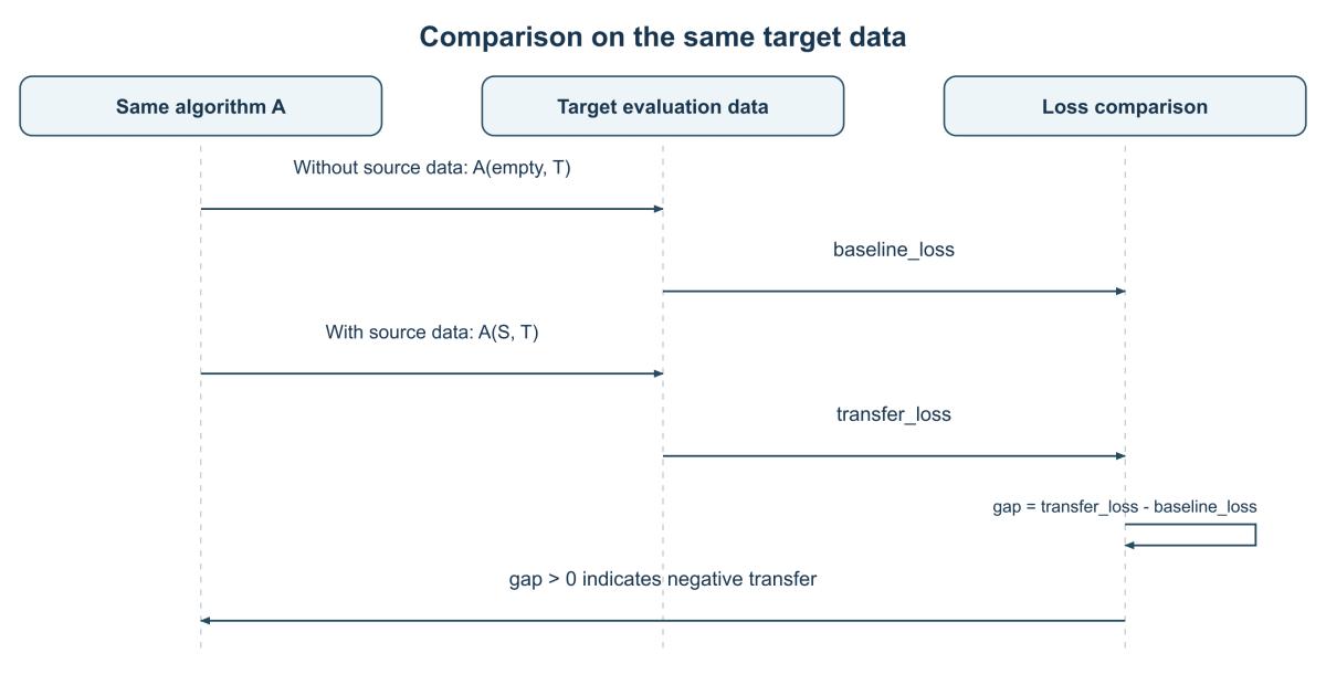
Both paths in the diagram are evaluated on the same target data under identical conditions. If the model architecture, optimizer, or target dataset size also changes between runs, the effect of those design changes must be separated from the effect of the source data.
Measuring degradation against a fixed baseline
Wang et al., Characterizing and Avoiding Negative Transfer (CVPR 2019), formalize negative transfer by fixing the learning algorithm and comparing the target expected risk of a model trained with source data, , against the same algorithm trained using only target data, 3. Comparing across different algorithms would confound the effect of the source data with differences between the algorithms themselves.

The excerpt above shows Equation (3) from Wang et al. (2019), §3 (page 2 of the authors’ arXiv preprint; source page). The left term is the target risk when source and target data are used together, and the right term is the target risk of the target-only baseline. Because risk measures expected loss (where lower is better), a strictly larger left-hand side—or equivalently a positive risk gap —indicates negative transfer.
Because true risk is an expectation over the target distribution, practical evaluations estimate it on finite validation or test samples. The table and the Python and C++20 examples below use synthetic numbers solely to illustrate the sign convention, not empirical measurements from a specific paper or LLM.
Target task loss | No source data | With source data | Change with source () |
|---|---|---|---|
Synthetic Case A | 0.10 | 0.06 | (lower loss, positive transfer) |
Synthetic Case B | 0.10 | 0.18 | (higher loss, negative transfer) |
Synthetic Case C | 0.10 | 0.10 | (no difference) |
- Target task loss
Synthetic Case A
- No source data $R_T(A(\emptyset, T))$
0.10
- With source data $R_T(A(S, T))$
0.06
- Change with source ($\Delta R_T$)
(lower loss, positive transfer)
- Target task loss
Synthetic Case B
- No source data $R_T(A(\emptyset, T))$
0.10
- With source data $R_T(A(S, T))$
0.18
- Change with source ($\Delta R_T$)
(higher loss, negative transfer)
- Target task loss
Synthetic Case C
- No source data $R_T(A(\emptyset, T))$
0.10
- With source data $R_T(A(S, T))$
0.10
- Change with source ($\Delta R_T$)
(no difference)
baseline_loss = 0.10
transfer_losses = [0.06, 0.18, 0.10]
# Compute R_T(A(S, T)) - R_T(A(empty, T)) under a fixed algorithm and target evaluation.
gaps = [round(loss - baseline_loss, 2) for loss in transfer_losses]
assert gaps[0] < 0
assert gaps[1] > 0
assert gaps[2] == 0
print(gaps)
Output:
[-0.04, 0.08, 0.0]Computing the same empirical risk gap in C++20 gives:
#include <array>
#include <iomanip>
#include <iostream>

int main() {
  constexpr double baselineLoss = 0.10;
  constexpr std::array<double, 3> transferLosses{0.06, 0.18, 0.10};

  std::cout << std::fixed << std::setprecision(2);
  for (std::size_t i = 0; i < transferLosses.size(); ++i) {
    // A positive gap indicates higher target risk (negative transfer) under fixed algorithm A.
    double gap = transferLosses[i] - baselineLoss;
    std::cout << gap << (i + 1 == transferLosses.size() ? '\n' : ' ');
  }
  return 0;
}
Output:
-0.04 0.08 0.00Here a positive gap () means adding source data increased target loss, which corresponds to negative transfer. If the evaluation metric is one where higher values are better—such as accuracy or score—the sign convention flips accordingly. Drawing reliable conclusions in practice requires accounting for training variance across random seeds and sample uncertainty on the evaluation set rather than judging from a single output.
What gets transferred is not a single mechanism
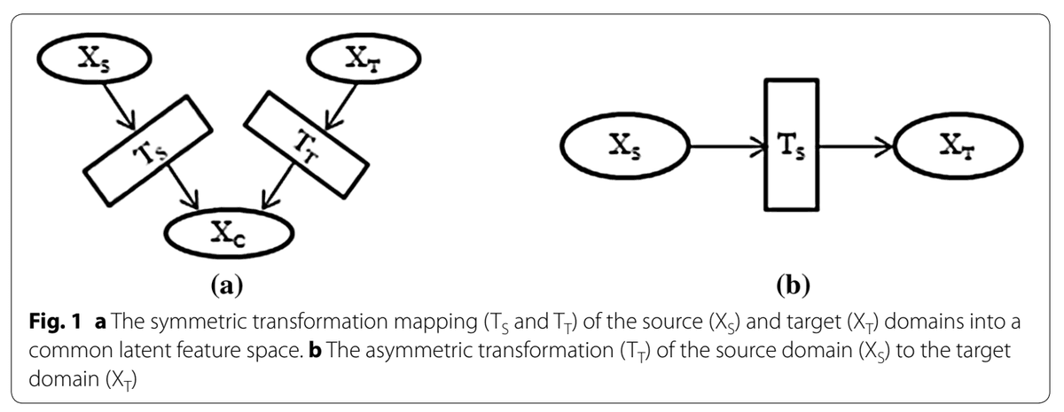
Figure 1 from Weiss, Khoshgoftaar, and Wang (2016), A survey of transfer learning, illustrates two designs for feature-based transfer4 (original figure, CC BY 4.0). Subfigure (a) maps both source and target domains into a common latent feature space (symmetric transformation), whereas (b) transforms features of one domain directly into the representation space of the other (asymmetric transformation). This diagram depicts feature-space domain adaptation rather than the gradient update graph of fine-tuning a pretrained language model.
Parameter transfer—as covered in Pretraining, fine-tuning, and in-context learning—differs in implementation from feature-space transformations and instance reweighting. Calling a procedure "transfer" does not by itself specify whether model weights were updated, a feature projection was learned, or demonstrations were supplied inside an inference prompt.
Near vs. far transfer and interference across tasks
Near transfer and far transfer describe how closely the structure and representation of a new evaluation setting resemble the training setting, whereas positive and negative transfer describe whether target performance improves or degrades. Even when two domains appear superficially close, differences in the conditional label distribution can still induce negative transfer.
Similarly, adapting a pretrained model to optimize a narrow reward or formatting constraint (such as aggressive compression in code or math) can improve the targeted objective while degrading performance on broader comprehension or writing tasks. In neural networks, this trade-off is closely tied to catastrophic forgetting (or catastrophic interference)5; testing whether adaptation to one domain causes negative transfer on another requires evaluating both tasks against the same pre-adaptation baseline.
See also
Footnotes
- Sinno Jialin Pan, Qiang Yang, “A Survey on Transfer Learning,” IEEE Transactions on Knowledge and Data Engineering 22(10), 2010, pp.1345–1359. Paper, DOI. ↩
- Michael T. Rosenstein, Zvika Marx, Leslie Pack Kaelbling, Thomas G. Dietterich, “To Transfer or Not to Transfer,” NIPS 2005 Workshop on Inductive Transfer: 10 Years Later, 2005. Paper. ↩
- Zirui Wang, Zihang Dai, Barnabás Póczos, Jaime Carbonell, “Characterizing and Avoiding Negative Transfer,” Proceedings of the IEEE/CVF Conference on Computer Vision and Pattern Recognition (CVPR), 2019, §3, Eq. (3). arXiv paper, DOI. ↩
- Karl Weiss, Taghi M. Khoshgoftaar, DingDing Wang, “A survey of transfer learning,” Journal of Big Data 3(9), 2016, Figure 1 (CC BY 4.0). Paper, DOI. ↩
- James Kirkpatrick et al., “Overcoming catastrophic forgetting in neural networks,” Proceedings of the National Academy of Sciences (PNAS) 114(13), 2017, pp.3521–3526. Paper, DOI. ↩